Big Peer
Ditto's distributed database architecture is a composition of Small Peers and Big Peers. Small peers are predominantly used to synchronize data across web, mobile, desktop, and IoT apps where storage, RAM, and CPU resources are generally static and unchangeable. For example, if you were to buy an iPhone with 256 Gigabytes of storage, you are pretty much stuck with this size unless you buy another iPhone.
Conversely, Big Peers are database peers which live in the cloud and are capable of sharding or partitioning. When they sync with small peers, they look like any other peer. However, a Big Peer can be split across multiple virtual or physical nodes allowing for both horizontal and vertical scaling of resources as your application demands grow.
The Big Peer fits into Ditto's vision of syncing data, anywhere. Big Peer is cloud-ready, multi-tenant, highly available, fault tolerant, offers causally consistent transactions, and works seamlessly with Small Peer devices.
For reference:
- Web, iOS, Android, Raspberry Pi, Desktop, and some server side apps 👉 Small Peer
- Ditto Cloud 👉 Big Peer
Why Did You Make It?
Even with the Small Peer's wireless mesh networking capabilities, some pair of devices may not be able to exchange data. Maybe the devices are miles apart, or they are never online at the same time. That is where Big Peer fits in. The Big Peer is a database that Small Peer devices can sync with to propagate changes across disconnected meshes, and even back to the enterprise. Often databases are used as channels, which is also one of Big Peer's purposes.
There exist many distributed databases, but Big Peer is specifically designed for Ditto: It stores Ditto's CRDTs by default; it can store and merge Ditto CRDT Diffs; it "speaks" Ditto's mesh replication protocol, meaning it appears as just another peer to Ditto mesh devices; and it provides causally consistent transactions.
How Does It Work?
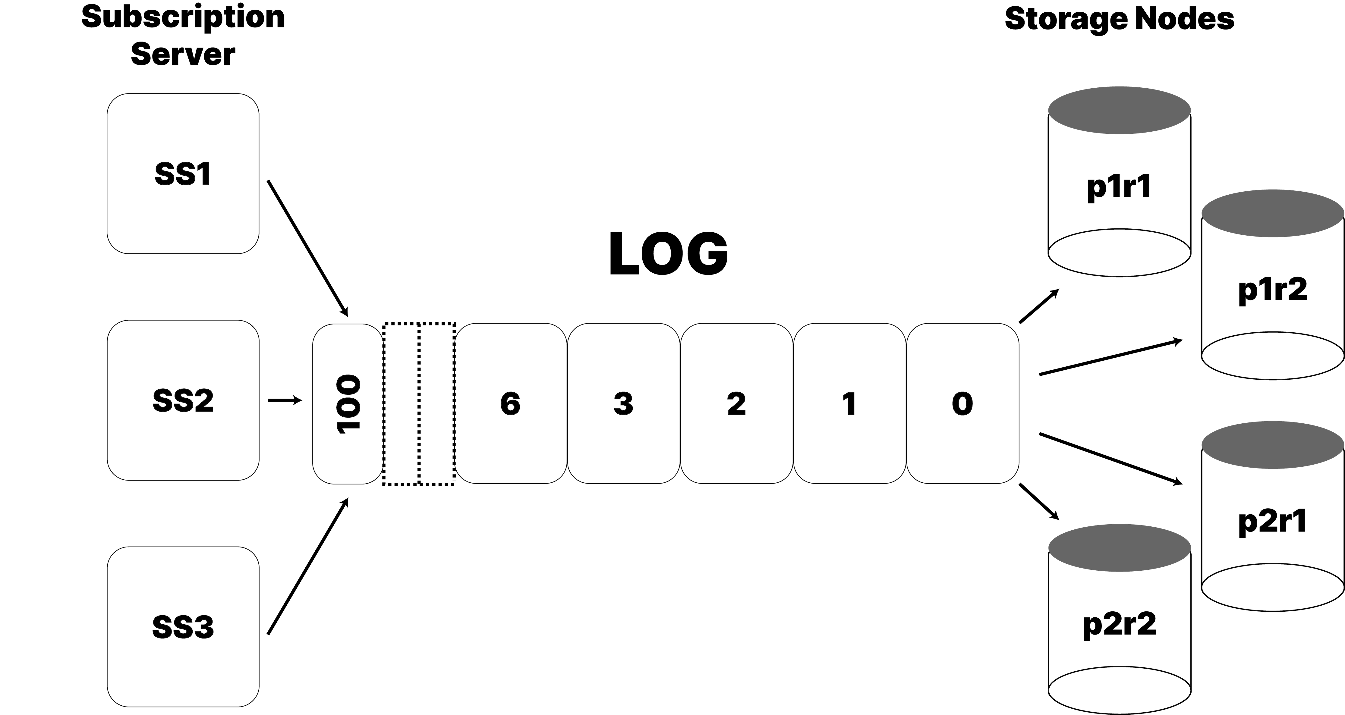
Big Peer is made up of core storage nodes which make a distributed database, and soft-state satellite API nodes, called Subscription Servers, that are also caches of data and replicate with Small Peer clients as a "Big Peer".
The following sections go into detail about what properties and features Big Peer has, and how we achieve those properties, leveraging our experience building and shipping distributed databases, and current computer science systems research.
The following drawing is a rough overview of the architecture.
Ditto CRDTs
The core data type in Ditto is the CRDT. It is documented in detail here. Understanding some of how CRDTs work helps understand the concepts below. It is enough to know that if the same CRDT is modified by multiple Ditto mesh Small Peer devices concurrently there is a way to deterministically merge the conflicting versions into a single meaningful value.
Ditto Mesh Replication
This is also covered in other documents. All we need know here is that Small Peer devices replicate with Big Peer by sending CRDT Documents and CRDT Diffs to Big Peer's Subscription Server API, and receive in return Documents and Diffs that they are subscribed to. A subscription is a query, for example "All red cars in the vehicles collection."
Thanks to the Ditto replication protocol, all Documents and Diffs that the client needs to send/receive to/from Big Peer appear to arrive atomically, as though in a transaction.
Apps and Collections
An application is the consistency boundary for Big Peer. An application is registered via the Portal. An application is uniquely identified via association with a UUID. Queries, Subscriptions, and Transactions are all scoped by application. Within an application are Collections. Theses are somewhat like tables, where associated Documents can be stored. Big Peer supports transactions within an Application, including across Collections.
Causally Consistent Transactions
Given the existence of the CAP theorem, which posits a fundamental trade off in distributed systems between Consistency and Availability in a world of asynchronous networks, Causal Consistency is the strongest consistency model that can be achieved if a system is designed to continue to be Available in the CAP sense. You can read more on Wikipedia.
Causal Consistency is a model that is much simpler to work with when compared to Eventual Consistency. Under Eventual Consistency, it seems like anything is allowed to happen. With Causal Consistency, if one action happens before another, and can therefore potentially influence that other action, then those two actions must be ordered that way for everyone. If two actions are totally unrelated, they can be ordered any way the system chooses. By way of example:
Imagine that you have two collections: Menus and Orders. First, you add a new item to the menu, and then create an order that points to the new item. If these two independent actions were re-ordered by an eventually consistent system, some devices could see that the menu item referenced in the order does not exist. Causal Consistency ensures that the menu item is added before the order is created, regardless of the vagaries of networks, connections, and ordering of messages. Transactional Causal Consistency means that we can apply this constraint across any number of related changes, across multiple documents, in multiple collections, as long as they are within the same Application. This is a much simpler to understand model compared to Eventual Consistency, leading to fewer surprises.
PaRiS - UST
This section gets technical on how Big Peer provides Causally Consistent Transactions, and other properties, like fault tolerance, and scalability.
The key concept throughout, and the primitive on which Big Peer is built, is that of the UST, the Universally Stable Timestamp. Along with some core architecture, the UST is inspired by the paper PaRiS: Causally Consistent Transactions with Non-blocking Reads and Partial Replication. The paper describes a system that very closely matches Ditto's needs. The system is a database, one that is partitioned (or sharded) to allow storage of a great deal of data, and replicated to provide fault tolerance (and better tail latencies/work distribution.) PaRiS supports non-blocking reads in the past, and causally consistent transactions. The key ingredient is the UST.
In PaRiS every write transaction is given a unique timestamp. All transactions that contain data for the same partitions will have a timestamp that is ordered causally. Non-intersecting transactions can have equal timestamps, as they have no causal relationship/order.
The key concept is that Transactions are ordered by Timestamp. Changes that have a causal relationship express their order relationship through the order of transaction timestamps. Transactions with no causal relationship can be ordered in any way. In the example above, as the change to the Menu collection happens before the changes to the Orders collection. The first would have a lower transaction ID than the second (if not part of the same transaction.)
Before going into more details about Ditto's implementation, some clarification on terms and concepts follows.
Replicas
Replicas are independent copies of the same data, which provide fault tolerance and better performance. For example, if there exist three replicas and a disk fails, two copies remain. If one or two replicas are unreachable due to network conditions, you can still read from a reachable one. Replicas improve performance by providing more capacity to serve reads. If you have three replicas you can balance reads across all three, each doing a third of the work. Data replication strategies (i.e., how data is replicated) have an effect on when you can read what.
As an initial look at the UST, imagine a database on a single machine with a transaction log. Each transaction to be written goes into the log and is given a sequence number. When the transaction is committed, the sequence number can represent the current version of the database. For example, when transaction with sequence number 1 is committed, the database is at Version 1. When the second transaction commits, the database is at Version 2, and so on.
Let's walk through a replication example to understand how reads work. Say we have two replicas of our data, A and B. Replica A commits Transaction 1, and then sends it to Replica B, who also commits it. Now the database is at Version 1, and both replicas will return the same answer. But what if Transaction 2 doesn't make it to Replica B? This can happen if there is a brief network outage, or for some reason the message is delayed. So while message B is delayed, A has committed transactions 1 and 2, but B only has committed Transaction 1. Since Ditto is causally consistent, it never blocks reads or writes. This means that a client can read even while replicas are in an inconsistent state.
If the system wishes to spread the read load equally, and a client reads from A, and after that reads from B, the client will see a non-consistent view of the world, where time goes backwards between the first read, and the second. However, we could decide that since only Version 1 is committed on both replicas, then the version of the database could be thought of as Version 1. This is the highest transaction that is committed on both replicas: the universally stable timestamp (UST). By enforcing reads to conform to the UST, clients reading from either replica will get a consistent view of the data.
Versions
The above scenario in "Replicas" suggests that we need to keep multiple versions of our data. If Transaction 1 changes documents A, B, and C, and Transaction 2 changes documents A, C, and F, BUT only one replica has stored both transactions, then the database is at Version 1. We therefore need to have the data for A and C at transactions 1 and 2, since if we want to provide a consistent view of the data (one that does not go back in time) then we can only serve reads as of Version 1 at first, and then later as of Version 2.
Big Peer keeps as many versions of each data item as it needs in order to provide consistent reads. If this concerns you, skip ahead to garbage collection.
Note that Big Peer uses Ditto CRDTs as the data type, meaning all
versions can be deterministically collapsed into one version, by
merging the CRDTs. In some cases a "version" is in only a Diff and not a whole document.
Partitions / Shards
In order to evolve the conceptual model we can add in partitioning of the data, or partial replication as it is called in the PaRiS paper. Often called Sharding, this is the practice of splitting up the key space of a database, and assigning a subset of it to different servers. See Random Slicing below for details of HOW we do this in Big Peer.
Now we have replicas of the data, and we partition the data. Each storage node in Big Peer is responsible for one replica of a data partition. If we want to split our data across three partitions, and have two replicas of each item, then we can deploy six servers, two in each partition.
Returning to our example in "Causally Consistent Transactions," imagine that the documents in the Menus Collection is stored in Partition 1, and the Orders Collection in Partition 2, and that the change to Menus and Orders occurs in the same transaction, Transaction 1.
This transaction contains documents that are stored in two different partitions, across a total of four locations (two replicas, two partitions).
In order to store the data for this transaction it needs to be stored on all four servers. This is why the UST matters. If, by chance, Big Peer stores the Orders change document before storing the Menus change document, and allow reads to always get the latest value, we can break the consistency constraint, and reference a menu item that doesn't exist.
A more complex example:
If we have four transactions in flight, maybe all the servers have committed Transaction 1, half have committed Transaction 2, all have committed Transaction 3, and only two servers have committed Transaction 4. If we want to have consistent read of the data, we have to read at the version that is stable at all servers: Transaction 1. Note: we can't say that Transaction 3 is stable, since it follows Transaction 2, which is not yet stable. Causal Consistency is all about the order of updates.
Non-Blocking Reads
When reading from Big Peer, you don't have to wait for the last write to become stable before reading. Instead, Big Peer is always able to return a version of the data for the UST. Reading in the past is still causally consistent, and it means that reads and writes proceed independently. It also means that something is always available to be read (given one replica per-partition is reachable)—a reasonable trade-off.
Read Your Own Writes
In the PaRiS paper, the database clients must have a local cache of their own writes, so that they can always read their own writes. In Ditto, the Small Peer clients are fully fledged partial replicas of the database, and can always read their own writes. For the HTTP API, writes return a Timestamp at which the write is visible. A HTTP Read request can provide this timestamp to ensure Read-Your-Own-Writes semantics.
The Log
A core concept in Big Peer is the log. We use a transaction log to propagate updates to the database. In PaRiS, a two-phase commit process is used to negotiate an HLC-based sequence number for each transaction. In Big Peer, we use the log to sequence transactions. The sequence number for a Transaction in the log becomes the Transaction Timestamp, which is what the UST reflects. The Transaction Timestamps in Big Peer form a total sequence, from ZERO (initial empty database version) on up. Each storage node consumes from the log, and a transaction is stable when all nodes have observed the transaction, those that own data in the transaction having written that data durably.
At present our log is Kafka, as it suits our needs well. Though Kafka
is at the heart of Big Peer, it is not a core architectural feature: any
log will do. At present, we use a single partition of a single topic,
but we can partition the log by Application and still maintain the
same consistency guarantees. When we do partition the log the properties are the
same, the throughput increases, and the UST becomes
a vector. Developers can register Kafka consumers
where Big Peer will deliver data change events that match a defined query -
similar to how Small Peers can observe queries to react to data changes.
Storage Nodes
Big Peer is split into Storage Nodes and Subscription Servers. The Storage Nodes are the database nodes, they run RocksDB as a local storage engine. A storage node consumes the transaction log, commits data to disk, and gossips with the other storage nodes.
Gossip - UST
Each node gossips the highest transaction that it has committed. From this gossip, any node can calculate what it considers to be the UST. If every server gossips its local MAXIMUM committed transaction, then the UST is the MINIMUM of those MAXIMUMS. For example, in a three-node cluster:
- Server 1 has committed Txn 10
- Server 2 has committed Txn 5
- Server 3 has committed Txn 7
The UST is "5".
NOTE: each server can have a different view of the UST, depending on how long it takes messages to be passed around. For example:
- Server 1 has committed Txn 10, and has heard from Server 2 that it has committed Txn 4, and from Server 3 that it has committed Txn 6. Server 1 thinks the UST is "4".
- Server 2 has committed Txn 5 and has heard from Server 1 that it has committed Txn 7, and from Server 3 that it has committed Txn 6. Server thinks the UST is "5"
- Server 3 has committed Txn 7 and has heard from Server 1 that it has committed Txn 9, and from Server 2 that it has committed Txn 3. Server thinks the UST is "3"
But whatever the view of the UST, it reflects a causally consistent version of the database that can be read.
When Big Peer is working, then the UST moves up. When Big Peer is quiescent the UST will be the same on every node, and will reflect the last transaction produced by the log.
The mechanism for gossip in Big Peer is the subject of future optimization work.
Gossip - Garbage Collection
Very similar to the UST is the Garbage Collection Timestamp. It works closely with Read Transactions (below). The Cluster GC Timestamp represents the lowest Transaction Timestamp that must not be garbage collected. The GC timestamp and the UST form a sliding window of versions over the database that represent the Timestamp versions at which a Causally Consistent query can be executed.
Document versions below the GC Timestamp can be garbage collected. Garbage Collection is a periodic process that scans some segment of the database, and rolls up, or merges all the versions below the GC timestamp, re-writing them as a single value. Thanks to Ditto CRDTs, this leads to a deterministic outcome value for each document at each version.
Garbage Collection keeps the number of versions to a minimum, making reads more efficient, and reclaiming disk space.
The Garbage Collection Timestamp is calculated as the minimum active Read Transaction Timestamp across the cluster.
Reading and Read Transactions
Queries are handled by a coordinating node. Any node can coordinate a query, because every node has a local copy of the Partition Map, from the Cluster Configuration. As such, the coordinator can be chosen at random, or via some other load balancing heuristic.
The node will look at the query and decide which partitions contain the data needed to answer the query. At present, Big Peer shards data by Application AND Collection (however this can change in the future). The coordinator will assemble a list of partitions needed to answer the query, and pick one replica from each partition. It picks the replica based on a fault-detector, picking the replica least likely to be faulted. It sends the query to each replica, and merges and streams the results back to the caller.
The Coordinator issues the query to each partition with a predetermined timestamp. This timestamp is usually the UST at the Coordinator, but can be any timestamp between the cluster Garbage Collection Timestamp and the UST.
When a node coordinates a Read Transaction, it locally holds some metadata in memory, indicating the value of the UST at the time the transaction began. This data is used to calculate the Local Garbage Collection Timestamp that the node gossips. The Local GC timestamp is the maximum transaction below the minimum read transaction. The GC timestamp proceeds monotonically upwards, as does the UST. When the query is complete, the Read Transaction is removed from memory, and the GC timestamp can rise.
A node that is not currently performing a Read Transaction will still gossip its view of the UST as the GC timestamp. This way progress can always be made.
In a quiescent cluster with no reads, the GC timestamp will equal the UST, and there will be exactly one version of each data item.
Cluster Configurations: Who owns what?
The details of the cluster: its size, shape, members, partitions, replicas etc. are all encapsulated in a Cluster Configuration. When there is a need to change a cluster, we create a new Cluster Configuration and instruct Big Peer to transition from the Current Configuration to the Next Configuration.
Everything discussed so far describes a static configuration of partitions and replicas. However, clusters must scale up and down, and faulty nodes must be removed and replaced. Big Peer must support dynamic scaling without downtime, and it must do so while maintaining Causal Consistency, always accepting writes and serving reads.
Ideally, when a cluster is changed, there should be minimal data movement. That is, if we grow the cluster, we want to only move the minimum amount of data necessary to the new nodes.
Before discussing Transitions in detail, it's helpful to look at how data is placed in a Big Peer cluster, and for that we use Random Slicing.
Random Slicing
Random Slicing has been written about brilliantly in this article by Scott Lystig-Fritchie, which motivates the WHY of Random Slicing as well as explaining the HOW. Here, we will briefly discuss Big Peer's implementation.
We made a decision to make this first version of Big Peer as simple as possible, and so we elected to keep our cluster shape and replica placement very simple (though it is extensible and will get richer as time allows or needs dictate).
Each document in Big Peer has a key, or document ID which is made up of a Namespace (The Application (AppId) and the collection) and an ID for the document. We hash a portion of this DocumentId (at present the Namespace) and that gives us a number. This number decides in which partition the data item lives. Our current hashing policy has the effect that data in the same Collection is co-located in the same partition, which makes queries in a single Collection more efficient. It may also lead to hot spots, but this can be mitigated by either hashing more of the DocumentId (to split Collections), or inserting a layer of indirection that allows us to map hot partitions to bigger nodes ("The Bieber problem": see the paper, or Scott's article for details.)
As per the Random Slicing algorithm, we think of the keyspace as the range 0 to 1. We take the capacity of the cluster, and divide 1 by it. This determines how much of the keyspace each partition owns.
In our initial, naive, implementation the capacity is the number of partitions we wish to have. We enforce an equal number of replicas per-partition, and thus all clusters are rectangular. E.g. 1*1, or 2*3, or 5*2, etc., where the first number is the number of partitions, and the second the number of replicas. Random Slicing allows in future to have heterogeneous nodes, assigning the capacity accordingly.
In the case that we want three partitions of two replicas, we say each partition takes 1/3 of the keyspace, or has 1/3 of the capacity.
Hashing a DocumentId then gives us a number that falls into the 1st, 2nd or 3rd 1/3 of the keyspace, and that decides which partition owns that document.
We can transition from any configuration to any other, and we do this by slicing or coalescing partitions using the Cut-Shift algorithm from the Random Slicing paper.
The graphic below illustrates how this looks.
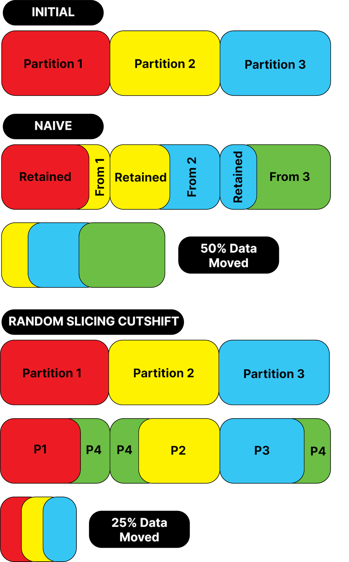
As the image shows, Partition 4 (P4) is made up of slices from P1, P2, and P3, these three slices we call Intervals. They represent, in this case, two disjoint ranges of the keyspace that P4 owns. A replica of P4 has two intervals, whereas P1 has a contiguous range and a single interval.
Our Random Slicing implementation is currently limited in that resources must be added and removed in the cluster in units equal to the desired replication factor. If you want to add a node, and your desired replication factor is two, you must add two nodes. This is not a limit inherent in Random Slicing, but a choice we made to speed up implementation. As Scott's article points out, Random Slicing matches your keyspace to your storage capacity, but that is it! It doesn't manage replica placement. More complex replica placement policies are coming, read Scott's article 😉
In short, Random Slicing appears very simple, map capacity to the range 0-1, and assign values to slices in that range. Cut-Shift is a great way to efficiently carve new smaller, partitions from slices of larger ones, and coalesce smaller slices into larger partitions when Big Peer scales up or down.
Each storage node uses the Random Slicing partitioning information to decide if it needs to store documents from any given transaction. If the Random Slicing map says that Server One owns Documents in the first Partition, then for each transaction Server One will store Documents whose IDs hash to the first partition.
Interval Maps - Missed Transactions - Backfill
Each storage nodes keeps a local data structure, stored durably and
atomically with the document data, that records what transactions the
node has observed. The structure is called the IntervalMap, and
represents what has been observed, in what slices of the keyspace.
For example, if a server is responsible for an interval of the
keyspace that represents the first third of the keyspace, the server
"splices" the observed transactions into the IntervalMap at that
interval.
Imagine Server 1 is responsible for Interval 1, it receives transactions
1..=100 from the log, it adds the data from those transactions to a local write
transaction with RocksDB. Then it splices the information into the IntervalMap,
that it has seen a block of transactions from 1..=100. We now say that the
base for Interval 1 is 100. Now the server stores this updated
IntervalMap with the data in a write transaction to RocksDB.
Next the server receives transaction 150..=200 from the log. Clearly the
server can detect that it has somehow missed transaction 101..=149. The server
can still observe and record the data from these new transactions, and splice
the information into the IntervalMap. The IntervalMap now has a base of
100 and a detached-range of 150..=200.
Any server with any detached ranges can look in the Partition Map to see if it
has any peer replicas, and ask them for the detached range(s). This is an
internal query in Big Peer. If a peer replica has some or all of the missing
transaction data, it will send it to the requesting server, who will splice the
results in the IntervalMap, and write the data to disk. This way a server can
recover any data it missed, assuming at least one replica stored that data. We
call this Backfill.
Nodes gossip their IntervalMaps, this is how the UST is calculated, and how Backfill replicas can be chosen.
Read on down to "Missed/Lost Data" if you want to know how the cluster continues to make progress and function in the disastrous case that all replicas miss a transaction.
The IntervalMap, gossip, Backfill, UST, Read Transactions, and the GC
timestamp all come together to facilitate "transitions", which is how Big Peer can
scale up and down, while remaining operational, available, and consistent.
Transitions
Also mentioned in Scott's article on Random Slicing is the fact that Random Slicing will not tell you how, or when, to move your data around if you want to go from one set of partitions to another.
In Big Peer we have the added problem that we must at all times remain Causally Consistent. Big Peer manages Transitions between configurations by leaning on those two primitives the UST and the GC Timestamp. The process is best explained with an example.
Using the diagram from the Random Slicing section, a walkthrough of the transition from the three-partition original cluster to the target four-partition cluster. In this case assume two replicas per partition, which means adding two new servers to the cluster.
There is a Current Config, that contains the intervals that make up the partitions 1, 2, and 3 mapped to the replicas for those partitions. The name p1r1 refers to the first replica of Partition 1, p2r2 the second replica of Partition 2, etc.
In the Current Config there are nodes p1r1, p1r2, p2r1, p2r2, p3r1, p3r2. Two new nodes are started, (p4r1, p4r2). A new Cluster Configuration is generated from the Current Configuration. This runs the Cut-Shift algorithm and produces a Next Configuration, with the partition map and intervals as-per the diagram above.
We store the Current Config, and the Next Config in a strongly consistent metadata store. Updating the metadata store causes the Current Config and Next Config file to be written to location on disk for each Big Peer Store node, and each node is signaled to re-read the configs.
The servers in p1-p3 are all in the Current Config, and the Next Config. The servers in p4 are only in the Next Config.
A server will consume from the log if it is in either config. Those in both configs will store data in all intervals they own in both configs. In our example each of the current config servers stores a subset of the current sub-interval of its current ownership in the next config. The new servers in p4 start to consume from the log at once, and gossip to all their peers in both configs.
Backfill, again
For example, we start the new servers when the oldest transaction available on the log is Txn Id 1000. They must Backfill from 0-1000 from the owners of their intervals in the Current Configuration. They use the Current Configuration to calculate those owners, and the IntervalMaps from gossip to pick an owner to query for data no longer on the log. Recall that the UST is calculated from the base of the IntervalMap but these new servers (only part of the new config) do not contribute to the UST until they have Backfilled.
Routing, and a UST per-Configuration
In the section on UST we described a scalar value, the Transaction Timestamp. In reality this value is a pair of the ConfigurationId and the UST. The ConfigurationId rises monotonically, the initial Configuration being ConfigId 1, the second ConfigId 2, etc.
This allows us to calculate a UST per-configuration. Before we began the transition the UST was (1, 1000). The UST may never go backwards (that would break Causal Consistency). After starting the new servers and notifying nodes about the Next Config, the UST in the Current Config is (1, 1000) and in the Next Config is (2, 0). During this period of transition the nodes in p4 cannot be routed to for querying. Only nodes in the Current Config can coordinate queries, and these nodes decide what Configuration to use for Routing based on the USTs in each of the Current and Next Config. We call this the Routing Config. It is calculated. And like everything else in Big Peer, it progresses monotonically upwards.
After the new nodes have Backfilled, and after some period of gossip, the UST in the Next Config arrives at a value that is >= the UST in the current config* so the servers in the Current Config will begin to Route queries using the Next Config. Recall that nodes gossip a GC timestamp that is based on active Read Transactions. A Read Transaction is identified by the Timestamp at which it began. For example (1, 1000) is a Read Transaction that began at UST 1000 in the Current Configuration. When all the replicas in the Current Configuration are Routing with the next configuration, (e.g., the Cluster GC timestamp is in the Next Configuration, (2, 1300)) the Transition is complete. Any of the nodes can store the Next Config into the Strongly Consistent metadata store as the Current Config. Each node is signaled, and eventually all will have a Current Config with ConfigId 2, and will forget metadata related to ConfigId 1. Furthermore, Garbage Collection will ensure that replicas drop data that they no longer own.
Throughout the transition, writes are processed, queries are executed, and the normal monotonic progress of the Cluster's UST and GC timestamp ensure that the new nodes can begin to store data at once, and will be used for query capacity as soon as they support Causally Consistent view of the data.
*(there are details elided here about how we ensure that the Next Config makes progress and catches up with the current, whilst ensuring the cluster still moves forward)
Handling Failure
There are many failure scenarios in any distributed system. Big Peer leans heavily on a durable transaction log for many failure scenarios, and replicated copies of data for many others. Safety in Big Peer (bad things never happen) has been discussed at length above, in UST, and Transitions, and how Causally Consistent reads occur. Liveness, however, depends on every replica contributing to the UST. The UST (and GC timestamp) are calculated from gossip from every node. If any node is down, partitioned by the network, slow, or in some other way broken, it impacts the progress of the cluster. Yes, Big Peer can still accept writes, and serve (ever staler) reads, but the UST won't rise, Transitions won't finish and GC will stall (leading to many versions on disk.)
It is possible in future that we make some changes to how the UST is calculated, and use a quorum of nodes from a partition, or the single highest maximum transaction from a partition. The trade-off being that query routing becomes more complex, and in the event that the node that set the UST high then becomes unavailable...something has to give in terms of consistency. These trade-offs are mutable, we can re-visit them, we favoured safety in the current iteration of the design.
If some nodes are keeping the UST down, and slowing or halting progress, the bad node(s) can be removed.
Bad Nodes
In this first iteration of Big Peer we have the blunt, expedient tool available to us of killing and removing a node that is bad. The process is simple. Update the Current Config to remove the offending node(s) and signal the remaining servers. They will immediately no longer route to that node, use that node in their calculations, or listen to gossip from that node. This is fine as long as at least one node in each partition of the map is left standing.
As soon as the offending nodes are removed the data is under-replicated. At once add replacement nodes by performing a transition as above. For example, imagine p1r2 has become unresponsive. Remove it from the Current Config, create a Next Config with a new server to take the place of p1r2, store the configs in the Strongly Consistent metadata store, and signal the nodes. The new node will begin to consume transactions and backfill, and the UST will rise etc.
Missed/Lost Data
As described in the first Backfill section, it is possible, with a long network incident and a short log retention policy, that some transactions are missed. If all the replicas for a partition miss some intersecting subset of transactions, that data has been missed, and it is lost. This should never happen. If it does, we don't want to throw away the Big Peer cluster, and all the good data. Progress must still be made. In this case each replica of the partition understands from the IntervalMaps that some transaction T has been missed. After doing a strongly consistent read of the metadata store, to check that no server in the next config exists that may have the data, the replicas agree unilaterally to pretend that really they did store this data, and they splice it into their IntervalMaps. The UST rises, and progress is made.
It is essential to understand this is a disaster scenario, and not business as usual, but disasters happen, and they should be planned for. We do everything we can to never lose data, including a replicated durable transaction log with a long retention policy.
Subscription Servers
These are soft-state servers that act as other Peers to Small Peers. They speak the Ditto replication protocol. Small Peers connect to the subscription server, and based on their subscription, the SubscriptionServer will replicate data. Taking from the Small Peer device data that Big Peer has not seen, and sending to the Small Peer device data Big Peer has that the Small Peeer device subscribes to, and has not seen.
Subscription Servers also provide an HTTP API for non-Small Peer clients.
Document Cache
In order to not be required to query Big Peer for all data requested by Small Peers, all the time, the Subscription Server maintains a sophisticated, causally consistent, in-memory cache of a data. The data it chooses to cache is based on the Subscriptions of the Small Peers connected to it. By routing devices to a Subscription Server by AppId, we increase the likelihood that the devices have an overlapping set of Subscriptions and share common data in the cache.
The document cache takes data from the mesh clients and puts it on the log as transactions. It also consumes from the log, so that it can keep the data in the cache up to date, without querying Big Peer. Any documents that it observes on the log, that are potentially of interest to the cache, must first be "Upqueried" from Big Peer to populate the cache. As a cache becomes populated Upqueries decrease in size and number.
As clients disconnect, if any data is no longer required in the cache, it is eventually garbage collected away.
CDC
Completing the cycle of data in Big Peer is CDC (Change Data Capture). Each transaction produces a Change Data Message containing the type of change (e.g., insert, delete, update) and the details of the change. CDC is a way for customer to react to data changes that occur from the mesh or elsewhere, or even to keep external legacy databases in sync with Big Peer.
Data from CDC is available from Kafka. Developers can register Kafka consumers where Big Peer will deliver data change events that match a defined query - similar to how Small Peers can observe queries to react to data changes.
We also provide webhooks to enable delivery of data within Big Peer into other systems or to build server-side logic that reacts to data change events - such as performing data aggregations that write back into Big Peer or triggering an email to a user based off an event from a Small Peer. These data change events fit into "serverless" patterns and will work with any "functions-as-a-service" (FaaS) systems, such as AWS Lambda or others.
Care is being taken to ensure the delivery of these events are reliable. Endpoints are able to persist a unique marker that corresponds to the event, and later restart events from that same marker onward so that events are not missed during periods of interruption.
HTTP API
For more information on how to use the HTTP API, see the HTTP documentation.